Meet Bob - a man on a mission to build passive income and retire young. He's read all the self-help books, and one of the main ideas that stuck with him was the concept of investing in property. So, Bob decides to learn everything there is to know about the real estate market.

One of the first things Bob does is make a list of features that he thinks might affect the price of a property. He includes things like the number of bedrooms, the living room size, the number of kitchens (because who doesn't love food?), and even the garden size. He goes out inquiring about property prices and collects information about 5 houses.

But Bob isn't satisfied with just making a list - he wants to actually analyze the data and see which features have the biggest impact on property prices. That's where I come in. Bob and I decide to team up and use Bayesian linear regression to really dig into the data and see what's going on.

Together, Bob and I embark on a journey of learning and discovery as we delve into the world of Bayesian linear regression. Will we be able to uncover the secrets of the real estate market? Will Bob finally be able to retire and live the dream of passive income and endless margaritas on the beach? Only time (and a lot of math) will tell.

October 28, 2022

14 minute read

NOTE: The code implementation (with interactive plots!) as discussed in the article can be found here.

Linear Regression

Bob: So, I want to find out how different features affect the price of a house. Any thoughts?
Me: Bob, have you ever heard of linear regression? It's like a hammer in a toolbox, simple yet effective.
Bob: Yeah, but it's really been a while since I've studied it.
Me: No problem, Bob. I'll give you a quick refresher on linear regression.

Linear regression is a common statistical method used for modeling the linear relationship between a response variable and one or more predictor variables. In a linear regression model, the response variable is modeled as a linear combination of the predictor variables. \[y = w_1 x_1 + ... + w_n x_n\] The coefficients represent the strength and direction of the relationship between the variables.

A common approach to estimating the coefficients in a linear regression model is through maximum likelihood estimation (MLE). MLE seeks to find the parameter values that maximize the likelihood of the data given the model. \[w* = \text{argmax}_w \ p(D | w)\] where \(w*\) is the optimal value for \(w\). While MLE is widely used and can provide good results, it has some limitations. One limitation is that MLE estimates can be sensitive to outliers in the data, leading to unstable and potentially biased estimates. In addition, MLE estimates are point estimates and do not account for uncertainty in the estimates themselves, making it difficult to quantify the uncertainty in the model predictions.

An alternative to MLE is the maximum a posteriori (MAP) estimate, which combines the MLE estimate with a prior distribution over the model parameters. This can be represented as \[w* = \text{argmax}_w \ p(w | D)\] Using the famous bayes theorem we can rewrite this as, \[w* = \text{argmax}_w \ \frac{p(D | w)p(w)}{p(D)}\] Since \(p(D)\) does not depend on \(w\), we can ignore the term in the denominator and finally get, \[w* = \text{argmax}_w \ p(D | w)p(w)\] The MAP estimate can help to mitigate the sensitivity of MLE to outliers and provides a way to incorporate prior knowledge about the model parameters into the estimation process. However, just like the MLE, the MAP estimate is still a point estimate and does not provide a full probabilistic characterization of the model parameters.

Introduction to Bayesian Linear Regression

Bob: That was good to know, but I want to know how confident I am about my estimates? Can you help me out with that?
Me: Of course, Bob! That's why we're here. Bayesian Linear Regression is like a crystal ball, it can tell you how confident you should be about different predictions, whether you're weightlifting or making real estate investments.

Bayesian linear regression (BLR) is a probabilistic approach to linear regression that addresses the limitations of MLE and MAP. instead of searching for a single set of fixed weights (i.e. a point estimate), we aim to find a relevant distribution of model parameters \((w)\) given a specific dataset \((D)\). This is represented by the conditional probability, \(p(w | D)\). Additionally, we assume that the model parameters have a prior distribution, \(p(w)\), which reflects our initial knowledge or belief about the values of the parameters.

With the data and prior distribution given, we can use the famous Bayes Theorem again to calculate the posterior distribution of the parameters. \[p(w | D) = \frac{p(D | w)p(w)}{p(D)}\] This represents our updated knowledge about the parameters after incorporating information from the data. This theorem is a fundamental part of Bayesian Linear Regression and is why it bears the name Bayesian.

Advantages

One advantage of BLR is that it provides a full probabilistic characterization of the model parameters, rather than just point estimates. This can be useful for quantifying uncertainty in the model predictions and for making informed decisions about the model. In addition, BLR can be more robust to outliers in the data, as the prior distribution can help to regularize the estimates and mitigate the sensitivity of the estimates to the data. BLR can also incorporate sequential learning, allowing for the updating of model parameters as new data becomes available without retraining our model on the previous data.

Disadvatages

However, BLR also has some limitations. One limitation is that the choice of the prior distribution can significantly influence the posterior distribution and the model predictions. Careful consideration must be given to the choice of the prior distribution in order to obtain reliable and meaningful results. In addition, computing the posterior distribution can be computationally intensive, especially for large datasets.

Computation of posterior distribution

Bob: Hey, I need to know how you actually find this posterior. So far all I've heard is a lot of talking and no action.
Me: No need to rush, Bob. We'll get there in good time.

There are various methods for determining the posterior distribution in Bayesian Linear Regression (BLR), including both closed-form solutions and Markov Chain Monte Carlo (MCMC) methods.

Closed-form solution

One of the closed-form solution method is when the likelihood and prior distributions are both normal. In that case, the posterior distribution also has a closed-form solution and can be computed analytically. This is due to the fact that the normal distributions form a conjugate pair, which allows us to calculate the posterior in closed-form. So lets look at the closed-form solution when both the prior and likelihoods are normal distribution. \[p(w|t) = \mathcal{N}(w | m_N, S_N)\] Here \(m_N = S_N(S_0^{-1}m_0 + \beta\Phi^Tt)\) and \(S_N^{-1} = S_0^{-1} + \beta\Phi^T\Phi\)

and \(m_N\) is the posterior mean, \(S_N\) is the posterior covariance matrix (or just the variance if we're dealing with single dimension), \(m_0\) is the prior mean, \(S_0\) is the prior covariance matrix, \(\beta\) is the noise precision parameter (representing the inverse variance of the noise that is inherently present in the data), \(\Phi\) represent the design matrix and \(t\) represents the target vector.

Bob: So, it's like a magic trick, we wave our hands, and poof! We have the posterior.
Me: Yeah, something like that, Bob. Though it's not magic, it's just math. I derived this using a result from the book Pattern Recognition and Machine Learning. And now, you too can make all your posterior dreams come true.

Theorem

Given a marginal Gaussian distribution for x and a conditional distribution for y given x in the form: \[p(x) = \mathcal{N}(x | \mu, \Lambda^{-1})\] \[p(y|x) = \mathcal{N}(y | Ax + b, L^{-1})\] the marginal distribution of y and the conditional distribution of x given y are given by \[p(y) = \mathcal{N}(y | A\mu + b, L^{-1} + A\Lambda^{-1}A^T)\] \[p(x | y) = \mathcal{N}(x | \Sigma\{ A^TL(y-b) + \Lambda \mu \}, \Sigma)\] where \(\Sigma = (\Lambda + A^TLA)^{-1}\).

To use this theorem for our case, we just substitute \(x = w, y = t, \mu = m_0, \Lambda^{-1} = S_0, A = \Phi, b = 0\) and \(L = \beta I\) and voila, we have the result!

Markov Chain Monte Carlo (MCMC) methods

Bob: What if I don't want to just assume a normal prior. My beliefs are way more complex than that!
Me: No problem, Bob! We can still use Bayesian Linear Regression with more general or complicated prior distributions. You can even use the ones that are hard to spell if you want.

When working with Bayesian Linear Regression, sometimes the prior and likelihood distributions may not follow a closed-form solution, or the assumption of normal distribution for prior may not hold. In such cases, Markov Chain Monte Carlo (MCMC) methods can be used to approximate the posterior distribution. These methods involve creating a Markov chain that has the target posterior distribution as its stationary distribution and then drawing samples from the chain to approximate the posterior.

Bob: That sounds great! How do we implement this in practice?
Me: Don't worry, Bob. We can use the PyMC3 library to easily perform approximate bayesian inference using MCMC methods. Now you can use whatever prior you want, no matter how weird it is.

Making Predictions

Bob: That sounds great, can we also use this model to predict the prices of new houses based on their features?
Me: Obviously! That is one of the key advantages of using Bayesian Linear Regression.

BLR allows us to make predictions by considering the probability distribution of the weight vector, w, rather than relying on a single point estimate. This means that we can make predictions using ALL possible values of w and assign different weights to each value based on its probability i.e. we're making a weighted prediction. This is exactly how we can account for the uncertainty and variability in the model, allowing for a more robust prediction. Since our entire goal has been to make predictions on new samples given our dataset, what we have been meaning to compute is \(p(t | X, t, \alpha, \beta)\) which can be expressed as a marginalization of the joint distribution of the target variable, t, and weight vector, w as follows: \[p(t | X, t, \alpha, \beta) = \int p(t | w, \beta) p(w | X, t, \alpha, \beta) dw\] Here \(p(w | X,t, \alpha, \beta)\) can be thought of as the weight assigned to different weight vectors that are being used to make the prediction.

Bob: Wow, that's pretty cool! So, we can make predictions using an infinite ensemble of regression models, is that right?
Me: Exactly, Bob! And you can use the predictive distribution for further analysis, such as computing the mean or variance of the predictions.
Bob: This seems difficult to calculate. Is there a closed-form solution?
Me: Sometimes there is, but we're in luck because there is a closed-form solution for our case where the posterior distribution is normal and the distribution of the target variable given w is also normal. Imagine if we had chosen a more complex prior, we might have to resort to using approximate methods such as MCMC which can be computationally expensive.

For our case of normal likelihoods and priors, the predictive distribution can be described as \[p(t | x, D, \alpha, \beta) = \mathcal{N}(t | m_N^T \phi(x), \sigma_N^2(x))\] where \(\sigma_N^2(x) = \frac{1}{\beta} + \phi(x)^T S_N \phi(x)\)

Implementation

Bob: Thank you for all the theoretical insights. But listen, I have this secret suspicion that the Matrix is watching us, and I don't want it to know what I'm up to. So, teach me how to create my own Bayesian Regression model from scratch. I have a concern that pre-existing libraries may be monitoring my activity.
Me: Sigh. Are you sure you want to go through the trouble? It's like trying to make a fancy cake from scratch when you can just buy one at the store.
Bob: I'm positive, I want to keep my Bayesian Regression recipe a secret, just like how my grandma used to make her famous meatballs.
Me: Alright Bob, but just remember, this isn't cooking class, it's gonna be a lot of code and math. Are you sure you're up for it?


def compute_posterior(x_train, y_train, m_0, S_0, beta=None):
    """
		Returns mean and covariance matrix of the posterior normal distribution
		
		Parameters
		----------
		x_train : Training data features
		y_train: Training data labels
		m_0: Prior normal distribution mean
		S_0: Prior normal distribution covariance matrix
		beta: precision parameter (1/variance) of the noise, defaults to None

		Returns
		-------
		m_N: Posterior normal distribution mean
		S_N: Posterior normal distribution covariance matrix
		"""
    
    N = x_train.shape[0]

    # Compute beta if not passed
    if beta is None:
        w_mle = np.linalg.inv(x_train.T @ x_train) @ x_train.T @ y_train
        beta_inv = np.linalg.norm(x_train @ w_mle - y_train)**2 / N
        beta = 1 / beta_inv

    # Compute posterior covariance matrix
    S_N_inv = np.linalg.inv(S_0) + beta * x_train.T @ x_train
    S_N = np.linalg.inv(S_N_inv)
    
    # Compute posterior mean
    m_N = S_N @ (np.linalg.inv(S_0) @ m_0 + beta * x_train.T @ y_train)
    
    return m_N, S_N, beta

The code above is taking in the prior distribution parameters and the training data, and returning the posterior distribution of the weights.
The code first checks if beta has already been calculated. If it hasn't, the code goes on to calculate it.
Next, the code uses the formulas we discussed before to compute the posterior covariance matrix and the posterior mean, the values that help us understand the uncertainty of our model's predictions.


def make_predictions(sample, m_N, S_N, beta):
	"""
		Returns mean and the covariance matrix of the predicted distribution

		Parameters
		----------
		sample: A single sample for which predictions are to be made
		m_N: The mean of the posterior normal distribution
		S_N: The covariance matrix of the posterior normal distribution

		Returns
		-------
		m_pred: The predicted mean of the sample
		S_pred: The predicted variance of the sample

		"""
	m_pred = sample @ m_N
	S_pred = 1 / beta + sample @ S_N @ sample.T

	return m_pred, S_pred

This prediction function takes in a sample for which predictions are being made, the distribution parameters and beta. It then uses a formula that we have previously discussed to determine the parameters of the posterior distribution. As the formula is straightforward, the code is simple to understand.

That's all there is to it! Congrats, we've just implemented a basic Bayesian Linear Regression algorithm.

Bob: Let's put this baby to test on the dataset I collected and see some sweet results!

Visualizations

Let's take a property with 3 bedrooms, 1500 sq cm living area size, 1 kitchen and 600 sq cm garden size and make predictions on that using the model we just trained.

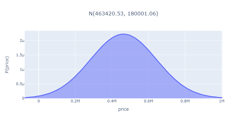
Wow, this house is looking at a price tag around a cool half mil, give or take a bit!
And it could even sell for something more or less as shown by the probabilities at different prices.

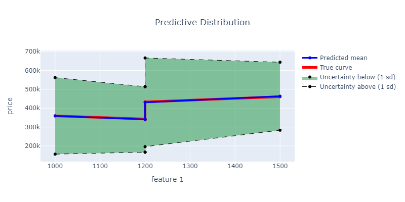
The plot shows that as the living room size increases, the property price also goes up.
The coefficients can also give an idea of how much the price changes with each unit of increase in living room size.

Bayesian Linear Regression